Néhémie’s Travelogue

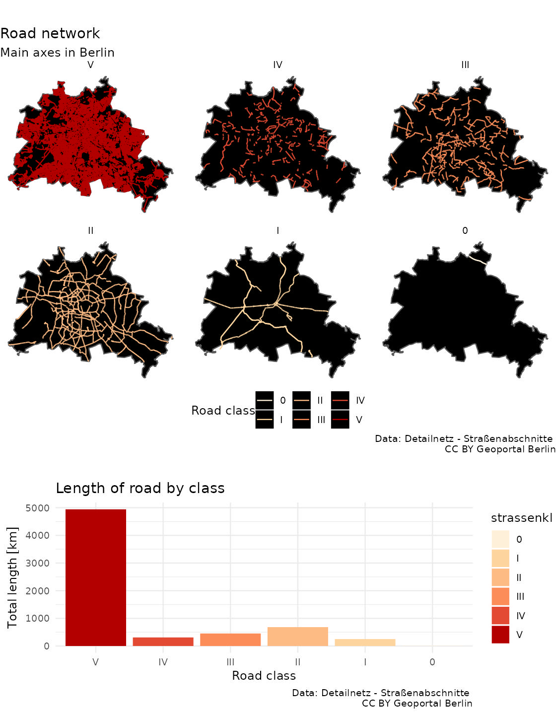
Yesterday I tried to give an overview of the road network of Berlin. Today, I would like to look a bit more into the difference between the road types. The length of each network is highly variable:

strassenkl	length [km]
V	4942
IV	309
III	453
II	683
I	251
0	10

Exhibit of the day

The same map as yesterday but each class is plotted separately. I also compute the length of each class network

Show the code of the exhibit

library(sf)
library(dplyr)
library(ggplot2)
library(units)

# "https://fbinter.stadt-berlin.de/fb/wfs/data/senstadt/s_vms_detailnetz_spatial_gesamt"
# https://tsb-opendata.s3.eu-central-1.amazonaws.com/detailnetz_strassenabschnitte/Detailnetz-Strassenabschnitte.gml
dsn <- read_sf("raw_data/Detailnetz-Strassenabschnitte.shp")
dsn$strassenkl <- factor(dsn$strassenkl)
dsn$strassenkl <- factor(dsn$strassenkl,
                            rev(levels(dsn$strassenkl)))
dsn$length <- st_length(dsn)

dsn_kl_length <- dsn %>% as.data.frame %>%
  group_by(strassenkl) %>%
  summarise(length = sum(length)) %>%
  mutate(length = set_units(length,km))

lor <- st_read("raw_data/lor_planungsraeume_2021.gml")
colnames(lor)[1:6] |> tolower() ->  colnames(lor)[1:6]
lor$plr_id <- lor$plr_id |> as.factor()
subset(lor, select=-bez) -> lor
lor_outer <- st_as_sf(st_union(lor))

p1 <- ggplot(dsn) +
  geom_sf(data=lor_outer, fill = "black") +
  geom_sf(aes(colour = strassenkl), lwd = 0.5) +
 facet_wrap(vars(strassenkl)) +
  theme_void() +
  theme(legend.position="bottom",
        legend.key = element_rect(fill = "black", colour =
                                  "white")) +
  labs(colour = "Road class") +
  scale_colour_brewer(palette="OrRd", limits = rev(levels(dsn$strassenkl))) +
  labs(title = "Road network",
       subtitle = "Main axes in Berlin",
       caption = "Data: Detailnetz - Straßenabschnitte \nCC BY Geoportal Berlin")

p2 <- ggplot(dsn_kl_length,
             aes(x= strassenkl, y= length)) +
  geom_col(aes(fill = strassenkl)) +
  theme_minimal() +
  xlab("Road class") +
  ylab("Total length")+
  scale_fill_brewer(palette="OrRd", limits = rev(levels(dsn$strassenkl))) +
  labs(title = "Length of road by class",
       caption = "Data: Detailnetz - Straßenabschnitte \nCC BY Geoportal Berlin")

library(gridExtra)
grid.arrange(p1, p2, ncol = 1)
# For saving only
gar <- arrangeGrob(p1, p2, ncol = 1,
                   heights = c(6, 3))
ggsave("2022-03-16_roads_by_class.jpg", gar,
       width=7.0,
       height=9,
       bg="white",
       dpi = 160)