Hierarchical Network

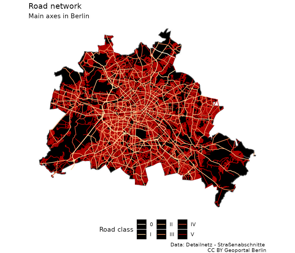
The classical way of organising a large network systems is to prioritize links to create a topological network. Roads are usually classified according to their functions and capacities. In Berlin, the City Development Plan (Stadtentwicklungsplan, abbr. StEP) is part of the urban planning to manage the spatial development of the city. A dedicated planning is reserved to mobility and transportation (Mobilität und Verkehr), that manage Berlin’s road network. On that page you can find a link to a document explaining the road classification quickly mentioned yesterday. Here some details about the classification:

0 = other

Continental road connection between metropolitan regions

I = large-scale connection

Connection between major centers in the region and the core areas

II = superordinate connection

Connection of core centers to the roads of level I, and connection to the large-scale transport system (airports, long-distance train stations, ports)

III = local connection

Connection between medium and local areas and connection to the regional transport system (regional train stations)

IV = supplementary road

Connection in residential and commercial areas as well as industrial areas

V = not part of the urban plan

Exhibit of the day

The same map as yesterday but with the main road coloured by classes

library(sf)
library(dplyr)
library(ggplot2)

# "https://fbinter.stadt-berlin.de/fb/wfs/data/senstadt/s_vms_detailnetz_spatial_gesamt"
# https://tsb-opendata.s3.eu-central-1.amazonaws.com/detailnetz_strassenabschnitte/Detailnetz-Strassenabschnitte.gml
dsn <- read_sf("raw_data/Detailnetz-Strassenabschnitte.shp")
dsn$strassenkl <- factor(dsn$strassenkl)
dsn$strassenkl <- factor(dsn$strassenkl,
                            rev(levels(dsn$strassenkl)))

lor <- st_read("raw_data/lor_planungsraeume_2021.gml")
colnames(lor)[1:6] |> tolower() ->  colnames(lor)[1:6]
lor$plr_id <- lor$plr_id |> as.factor()
subset(lor, select=-bez) -> lor
lor_outer <- st_as_sf(st_union(lor))

ggplot( dsn) +
  geom_sf(data=lor_outer, fill = "black") +
  geom_sf(aes(colour = strassenkl), lwd = 0.5) +
  theme_void() +
  theme(legend.position="bottom",
        legend.key = element_rect(fill = "black", colour =
                                  "white")) +
  labs(colour = "Road class") +
  scale_colour_brewer(palette="OrRd", limits = rev(levels(dsn$strassenkl))) +
  labs(title = "Road network",
       subtitle = "Main axes in Berlin",
       caption = "Data: Detailnetz - Straßenabschnitte \nCC BY Geoportal Berlin")

ggsave("2022-03-15_detailnetz_class.jpg",
       width=7.0,
       height=6,
       bg="white",
       dpi = 160)

Berlin’s map of main road network coloured. Data: CC BY “Geoportal Berlin / Detailnetz Straßenabschnitte”. Plot made with R, sf and ggplot2.